Y = Time to PPL (Hours)X = Student Age Group
49.4 15-19
40.8 15-19
69.2 15-19
56.7 15-19
52.5 15-19
54.1 15-19
55.4 15-19
79.3 15-19
45.7 15-19
60.4 15-19
48.3 15-19
55.8 15-19
44.6 15-19
58.8 15-19
55.2 15-19
50.6 15-19
59.8 15-19
60.3 15-19
73.6 15-19
77.3 15-19
84.4 15-19
48.9 15-19
58.3 15-19
66 15-19
62.8 15-19
57.3 15-19
71.8 15-19
74 15-19
58.1 15-19
96.7 15-19
75.2 15-19
53.5 15-19
53.4 15-19
58.1 15-19
69.6 15-19
68 15-19
53.5 15-19
82.8 15-19
75 15-19
73.1 15-19
100.2 15-19
55.9 15-19
59.5 15-19
67.8 15-19
61.2 15-19
72 15-19
49.4 15-19
70.7 20-29
72.1 20-29
36.4 20-29
39.5 20-29
42.8 20-29
43.4 20-29
43 20-29
41 20-29
59.5 20-29
43.3 20-29
53.7 20-29
44.2 20-29
50.2 20-29
45.8 20-29
46.4 20-29
42.9 20-29
51.2 20-29
42.7 20-29
50.1 20-29
48.1 20-29
41 20-29
48.3 20-29
54.9 20-29
86 20-29
100.9 20-29
59.4 20-29
50.1 20-29
48.5 20-29
44.7 20-29
47.1 20-29
47.2 20-29
42.6 20-29
58.6 20-29
49.1 20-29
56 20-29
44.9 20-29
48.6 20-29
43.7 20-29
45.6 20-29
59.1 20-29
53.5 20-29
56.2 20-29
45.5 20-29
52.3 20-29
54.4 20-29
54.2 20-29
50.7 20-29
50 20-29
47.2 20-29
61.3 20-29
60.4 20-29
50.3 20-29
52.9 20-29
58.6 20-29
61.7 20-29
54.3 20-29
51.2 20-29
60.9 20-29
55.3 20-29
46.9 20-29
50.2 20-29
51.2 30–39
52.5 30–39
73.1 30–39
71.8 30–39
41.5 30–39
41.7 30–39
44 30–39
42.8 30–39
48.9 30–39
61.6 30–39
48.1 30–39
52.7 30–39
38.4 30–39
54.6 30–39
48.3 30–39
53.5 30–39
57 30–39
52.9 30–39
49 30–39
45.9 30–39
51.4 30–39
55.1 30–39
45.4 30–39
61.9 30–39
50.1 30–39
49.4 30–39
46.8 30–39
63.1 30–39
62.4 30–39
57.2 30–39
53.8 30–39
62.4 30–39
46.3 30–39
51.3 30–39
50.2 30–39
59.1 30–39
72.5 30–39
70.5 30–39
56.2 30–39
56.7 30–39
55.7 30–39
63.4 30–39
51.8 30–39
50.1 30–39
50.5 30–39
55.7 30–39
60.8 30–39
43.9 30–39
56 30–39
59.1 30–39
59.8 30–39
49.7 30–39
54.5 30–39
52.8 30–39
77 30–39
56.9 30–39
49.7 30–39
69.8 30–39
73.8 30–39
61.8 30–39
44.2 30–39
78.5 30–39
80.6 30–39
52.3 30–39
51.9 30–39
54.4 30–39
65.3 30–39
56.3 30–39
60.4 30–39
62.7 30–39
78.3 30–39
58.5 30–39
67.8 30–39
65.6 30–39
56.8 30–39
73.8 30–39
86.7 40-49
61 40-49
60.7 40-49
64.1 40-49
56.2 40-49
67.1 40-49
73.1 40-49
70.5 40-49
79.1 40-49
59.9 40-49
74.6 40-49
64.3 40-49
78.9 40-49
72.4 40-49
59.2 40-49
63.3 40-49
68.7 40-49
75.2 40-49
67.5 40-49
67 40-49
68.5 40-49
115.6 40-49
72.3 40-49
53.8 40-49
61 40-49
57.4 40-49
66.7 40-49
59.9 40-49
61 40-49
54.3 40-49
63.2 40-49
61.3 40-49
71.1 40-49
66.7 40-49
63.6 40-49
62.4 40-49
54.7 40-49
70.4 40-49
53.7 40-49
62.9 40-49
44.8 40-49
76.6 40-49
67.2 40-49
61.7 40-49
64.1 40-49
46.4 40-49
80.5 40-49
85.7 40-49
74.3 40-49
90.4 40-49
59.5 40-49
77.3 40-49
84 40-49
83.9 40-49
97.1 40-49
70 40-49
74.5 40-49
80.3 40-49
70.3 40-49
64.5 50 or older
77.5 50 or older
69.8 50 or older
89.9 50 or older
75.3 50 or older
78.2 50 or older
89 50 or older
85 50 or older
81.3 50 or older
80.5 50 or older
84 50 or older
40 50 or older
82.4 50 or older
53.8 50 or older
101.4 50 or older
Week 2
Hypothesis Testing and Follow-up Tests with One-Way between Groups ANOVA
Graded Assignment
This week’s graded assignment is an application of the one-way ANOVA. The application
involves comparing the time (in hours) to earning a private pilots license (PPL) among different
age groups of flight students. The data were acquired from a random sample of N = 258 flight
students who completed their PPL at FIT Aviation. The data set for this assignment is located in
the Excel file “Week 2 Graded Assignment Data.” You are to import this data set into your
software program and do the following (see also the Week 2 Guided Example). Keep in mind
that fewer hours to PPL is “better” than more hours. This is analogous to the game of golf where
we strive for a low “score.”
A. Pre-Data Analysis
1. What is the research question?
2. What is the corresponding research methodology/design and why is this
methodology/design appropriate?
3. Conduct an a priori power analysis to determine the minimum sample size needed. Is the
given data set sufficient relative to this minimum sample size? In what way do you think
the size of the given sample will impact the results?
B. Data Analysis
Using the data from the Excel file, conduct a hypothesis test as follows:
1. Formulate the null and alternative hypotheses in symbols and words.
2. Determine the test criteria.
3. Test for the assumptions of ANOVA.
4. Run the analysis and report the results in an ANOVA summary table.
5. Make a decision to reject or fail to reject the null hypothesis and write a concluding statement.
C. Post Hoc Tests
If the omnibus is significant:
1. Summarize the results of the pairwise comparisons based on Tukey’s HSD in a table.
2. Interpret those comparisons that are statistically significant.
D. Post-Data Analysis
1. Report and interpret both of the effect size indexes, η2 and f.
2. Determine and interpret the power of the study.
3. Determine and interpret the 95% confidence intervals of the pairwise comparisons that are
significant and comment on the corresponding AIPEs.
4. Present at least one plausible explanation for the results.
m. of Aggressive
Hours
Behaviors
of Sleep
Observed
Deprivation
0 0 Hours
1 0 Hours
0 0 Hours
3 0 Hours
1 0 Hours
2 0 Hours
4 0 Hours
2 0 Hours
1 12 Hours
3 12 Hours
2 12 Hours
2 12 Hours
4 12 Hours
6 12 Hours
3 12 Hours
4 12 Hours
5 24 Hours
4 24 Hours
7 24 Hours
8 24 Hours
6 24 Hours
3 24 Hours
2 24 Hours
5 24 Hours
7 36 Hours
1 36 Hours
6 36 Hours
9 36 Hours
10 36 Hours
12 36 Hours
8 36 Hours
7 36 Hours
Week 2
Applying One-Way between Groups ANOVA
Guided Example
This handout material provides a guided example of the one-way between groups ANOVA.
Prior to working through this example you are strongly encouraged to read Chapter 11 (pp. 252–
278) of the assigned textbook by Wilson and Joye. You also should review the Gallo supplement.
The structure of this example will follow the structure used in previous guided examples.
Guided Example Context
The context of this guided example is the sleep deprivation study, which was presented in
Week 1’s Graded Assignment. Instead of examining this study from the perspective of the logic of
ANOVA, we now will include data that were collected from implementing the study and analyze
the data using ANOVA. As a convenience to the reader, the research description is replicated here
along with the corresponding data:
A common assumption is that sleep deprivation influences aggression. To test this
assumption a group of volunteer flight attendants were randomly assigned to sleep
deprivation periods of 0, 12, 24, and 36 hours, and then tested for aggressive behavior
in a controlled work environment involving pilots and passengers. The researchers then
observed the flight attendants’ behavior as they interacted with pilots and passengers
during the study period and recorded the total number of different aggressive behaviors
such as verbal “put downs,” getting into an argument, or verbal interruptions.
Hours of Sleep Deprivation
(Y)
Number of
Aggressive
Behaviors
Observed
Michael A. Gallo © 2019
0 Hours
24 Hours
48 Hours
72 Hours
0
1
0
3
1
2
4
2
1
3
2
2
4
6
3
4
5
4
7
8
6
3
2
5
7
1
6
9
10
12
8
7
Week 2: Guided Example: Applying One-Way ANOVA Page 1
Pre-Data Analysis
Before we engage in our traditional pre-data analysis activities, we first need to prepare
the given data set so that it is in a form that lends itself to being analyzed via ANOVA. The
corresponding Excel file titled “Week 2 Guided Example Data” reflects this form. Let’s now
address the pre-data analysis activities of stating the research question, identifying the correct
research methodology to answer the RQ, and conducting an a priori power analysis to determine
the minimum sample size needed based on a power of .80, a medium effect size, and an alpha
level of α = .05.
What is the RQ? The overriding research question for the current example is: “What is
the difference in the mean number of aggressive behaviors across the four levels (groups) of
sleep deprivation?”
What is the research methodology? The research methodology/design that would best
answer this question is true experimental. This is because the volunteer sample of flight
attendants is being randomly assigned to one of four treatment groups: 0, 12, 24, and 36 hours of
sleep deprivation, respectively.
What is the minimum sample size needed? To determine the minimum sample size, we
consult G•Power using the following parameters:
• Test family = F tests.
• Statistical test = ANOVA: Fixed effects, omnibus, one-way.
• Type of power analysis = A priori: Compute required sample size—given α, power,
and effect size.
• Input parameters are Effect size f = 0.25 (medium effect), α error prob = .05, Power =
.80, and Number of groups = 4. The minimum total sample size is N = 180.
Note that the given data set has a total sample size of N = 32, which is far fewer than the
minimum needed. This means there will be less than an 80% chance of correctly rejecting the
null hypothesis if the effect size in the sample data is f = 0.25. However, further note that if we
were increase the effect size to f = .65, then the minimum sample size is now N = 32. (Recall our
needle vs. basketball in a haystack analogy.) One justification for using a larger effect size is that
it is reasonable to expect a large effect size relative to the given context of sleep deprivation.
From our own personal experiences we know that the more sleep deprived we are the more likely
we are to be grumpy and irritable, and therefore we expect a large difference in the group means.
Michael A. Gallo © 2019
Week 2: Guided Example: Applying One-Way ANOVA Page 2
Data Analysis
We now conduct the hypothesis test. Following is a summary of the steps associated with
the corresponding hypothesis test.
Step 1: Formulate the null and alternative hypotheses.
Ho: µ0 hours = µ12 hours = µ24 hours = µ36 hours
(There will be no significant difference in group means across the four treatment groups.)
H1: At least one group mean is different from the others.
Step 2: Determine the test criteria.
• The test statistic is F.
• The level of significance is α = .05.
• The boundary of the critical region is determined from Table 2.1a given in the Gallo
Supplement from Week 2. Recall that the dfNum = (G – 1) and dfDen = (N – G). With a
given sample size of N = 32 and number of groups equal to G = 4:
— dfNum = (G – 1) = (4 – 1) = 3
— dfDen = (N – G) = (32 – 4) = 28
Therefore, the critical F will be based on df = (3, 28) and α = .05. However, because
Table 2.1a does not have an entry for dfDen = 28, we will use dfDen = 30. Therefore, the
critical F is F(3, 28) ≈ 2.92 as shown below.
α = .05
F(3, 28) ≈ 2.92
Step 3: Collect data and compute sample statistics. We first import the given Excel
file into our statistical software program. We next check to see if the data satisfy the underlying
assumptions of ANOVA. We then conduct a hypothesis test.
Checking assumptions.
• Independence. Because the flight attendants were randomly assigned to one of four
treatment groups, we assume the scores within each group are independent of each other.
Michael A. Gallo © 2019
Week 2: Guided Example: Applying One-Way ANOVA Page 3
• Normality. After examining each group’s q-q plot and respective Goodness-of-Fit tests,
all four groups are compliant with the normality assumption. (Note to the reader: You
should confirm this on your own.)
• Equal variances. Examining the Levene result for equal variances test, we get p =
.3472, which is greater than the preset alpha of α = .05. Therefore, the homoscedasticity
of variances assumption is met.
These preliminary considerations confirm that the assumptions are satisfied. As a result, we now
run the ANOVA. A copy of the corresponding ANOVA summary table is given below.
Source
SS
df
MS
F
Significance (p)
Between Groups
154.125
3
51.375
10.84
< .0001
Within Groups
132.750
28
4.741
Total
286.875
31
Step 4: Make a decision and a concluding statement.
Because F(3, 28) = 10.84 is greater than the corresponding F critical of 2.92, and p < .0001,
which is less than the preset alpha of α = .05, we reject the null hypothesis and conclude that at
least one group mean is significantly different than the other group means. Because the omnibus
test is significant, we may now conduct post hoc comparisons.
Post Hoc Tests
The results of the post hoc pairwise comparisons using Tukey’s HSD are summarized in the
table below.
Group Comparisons
MDiff
Std ErrDiff
95% CI
p
36 hours − 0 hours
5.875
1.09
[2.90, 8.85] < .0001
36 hours − 12 hours
4.375
1.09
[1.40, 7.35]
.0021
24 hours − 0 hours
3.375
1.09
[0.40, 6.35]
.0215
36 hours − 24 hours
2.500
1.09
[-0.47, 5.47]
.1231
24 hours − 12 hours
1.875
1.09
[-1.10, 4.85]
.3315
12 hours – 0 hours
1.500
1.09
[-1.47, 4.47]
.5232
Observe from the table that three of the six pairwise comparisons are statistically significant:
• Flight attendants who were sleep deprived for 36 hours had on average nearly 6 more
aggressive behaviors than flight attendants who were not sleep deprived (0 hours). This
5.875-unit mean difference was significant, p < .0001, 95% CI = [2.90, 8.85].
Michael A. Gallo © 2019
Week 2: Guided Example: Applying One-Way ANOVA Page 4
• Flight attendants who were sleep deprived for 36 hours had on average 4.375 more
aggressive behaviors than flight attendants who were sleep deprived for 12 hours. This
4.375-unit mean difference was significant, p = .0021, 95% CI = [1.40, 7.35].
• Flight attendants who were sleep deprived for 24 hours had on average 3.375 more
aggressive behaviors than flight attendants who were not sleep deprived (0 hours). This
3.375-unit mean difference was significant, p = .0215, 95% CI = [0.40, 6.45].
Although the mean differences of the other three pairwise comparisons were nonzero—for
example, flight attendants who were sleep deprived for 36 hours averaged 2.5 more aggressive
behaviors flight attendants who were sleep deprived for 24 hours—these mean differences were
not statistically significant.
Post-Data Analysis
We now determine, report, and interpret the corresponding effect size, power, and 95%
confidence intervals. We also discuss plausible explanations for the results.
What is the effect size? Recall that we report both η2 and f.
• η2 = .537, which means that approximately 53.7% of the variance in aggressive
behaviors is being explained by the comparison of the four sleep-deprived treatment
groups of 0, 12, 24, and 36 hours.
• To get f (as well as power) we consult G*Power and conduct a post hoc power analysis
by (a) changing the type of power analysis to Post hoc, (b) clicking on “Determine” to
open a side “drawer” to the right of the main window, (c) selecting “Effect size from
variance” under the “Select procedure in the side drawer, (d) clicking on the “Direct”
radio button, (e) entering the partial η2 that is reported by SPSS; and (f) clicking on
“Calculate and transfer to main window.” After completing these steps, G*Power
reports an f index of 1.076953. Thus, based on Cohen’s (1992) guidelines, this is a
large effect.
What is the power of the study? To determine the actual power of the study we simply
continue with G*Power by entering the total sample size (N = 32), α = .05, and Number of
groups = 4. When we click on “Calculate,” the corresponding power of the analysis is .999.
Thus, there is a greater than 99% probability that we made a strong correct decision to reject the
null hypothesis. In other words, there is a greater than 99% chance that the effect we found in the
sample truly exists in the population.
Michael A. Gallo © 2019
Week 2: Guided Example: Applying One-Way ANOVA Page 5
What are the corresponding 95% confidence intervals? For one-way ANOVA, we
report the 95% CIs as part of the post hoc comparisons (assuming the omnibus is significant). This
was done earlier. As for interpreting these intervals, we generally interpret only those associated
with the significant pairwise comparisons. As a result, we would interpret the first three 95% CIs
given in the pairwise comparison table:
• 36 hours vs. 0 hours: 95% CI = [2.90, 8.85], which means that 95% of the time we can
expect flight attendants who are sleep deprived for 36 hours to average as few as 2.9
more aggressive behaviors to as many as 8.85 more aggressive behaviors than flight
attendants who are not sleep deprived (0 hours).
• 36 hours vs. 12 hours: 95% CI = [1.40, 7.35], which means that 95% of the time we
can expect flight attendants who are sleep deprived for 36 hours to average as few as
1.4 more aggressive behaviors to as many as 7.35 more aggressive behaviors than
flight attendants who are sleep deprived for 12 hours.
• 24 hours vs. 0 hours: 95% CI = [0.40, 6.45], which means that 95% of the time we can
expect flight attendants who are sleep deprived for 24 hours to average as few as 0.4
more aggressive behaviors to as many as 6.45 more aggressive behaviors than flight
attendants who are not sleep deprived (0 hours).
Observe that all these 95% CIs are fairly wide, which means their respective accuracy in
parameter estimation (AIPE) is not that great. In other words, although the sample data provided
strong enough evidence to claim statistically significant differences in the group means for each
of these three pairwise comparisons, the data were not that compelling to provide us with an
accurate estimation of the true differences in these respective group means in the population.
What are some plausible explanations for the result? One plausible explanation is the
obvious: being sleep deprived takes a toll on our behavior. A second plausible explanation is
sample selection. Although flight attendants were randomly assigned to treatment groups, they
were not randomly selected. Therefore, this represents a selection threat to internal validity. A third
plausible explanation is the manner in which the observations were made. There was no
information in the research description about how aggressive behaviors were measured or who
measured them. For example, were they self-reported, did the researcher make the observations and
record them, was more than one person involved in observing/recording the data? This lends itself
to an investigator and/or instrumentation threat to internal validity.
Michael A. Gallo © 2019
Week 2: Guided Example: Applying One-Way ANOVA Page 6
Essay Writing Service Features
Our Experience
No matter how complex your assignment is, we can find the right professional for your specific task. Achiever Papers is an essay writing company that hires only the smartest minds to help you with your projects. Our expertise allows us to provide students with high-quality academic writing, editing & proofreading services.
Free Features
Free revision policy
$10Free bibliography & reference
$8Free title page
$8Free formatting
$8How Our Dissertation Writing Service Works
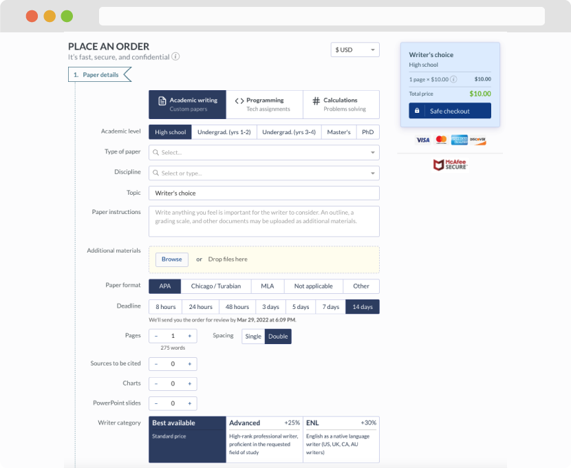
First, you will need to complete an order form. It's not difficult but, if anything is unclear, you may always chat with us so that we can guide you through it. On the order form, you will need to include some basic information concerning your order: subject, topic, number of pages, etc. We also encourage our clients to upload any relevant information or sources that will help.
Complete the order form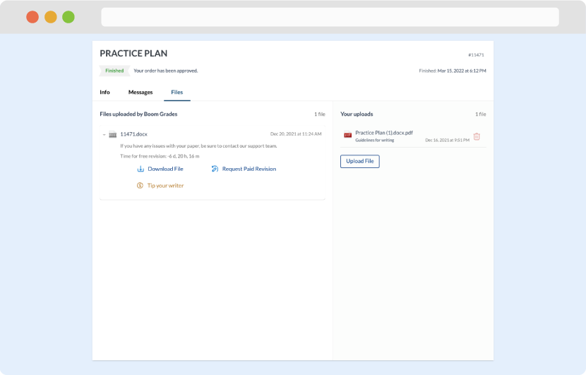
Once we have all the information and instructions that we need, we select the most suitable writer for your assignment. While everything seems to be clear, the writer, who has complete knowledge of the subject, may need clarification from you. It is at that point that you would receive a call or email from us.
Writer’s assignment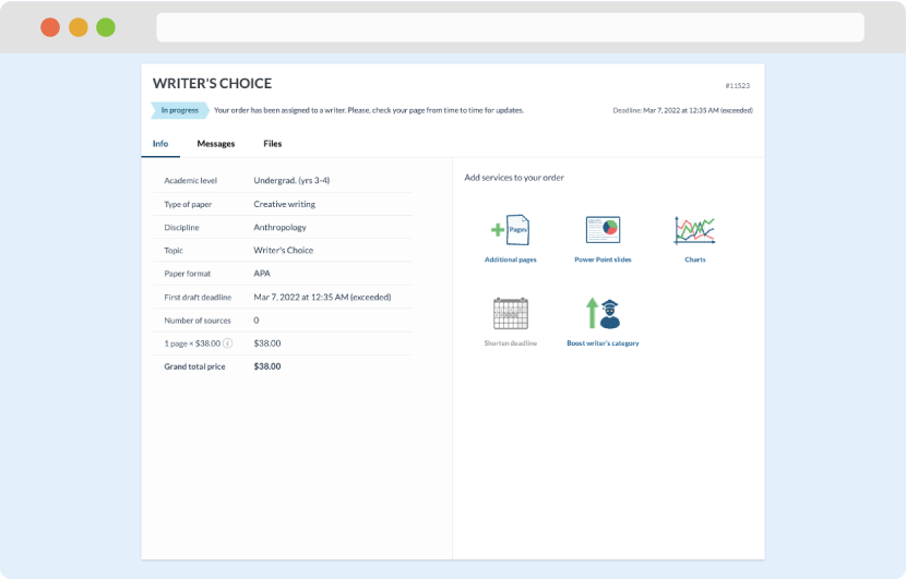
As soon as the writer has finished, it will be delivered both to the website and to your email address so that you will not miss it. If your deadline is close at hand, we will place a call to you to make sure that you receive the paper on time.
Completing the order and download